14. Graph Pane
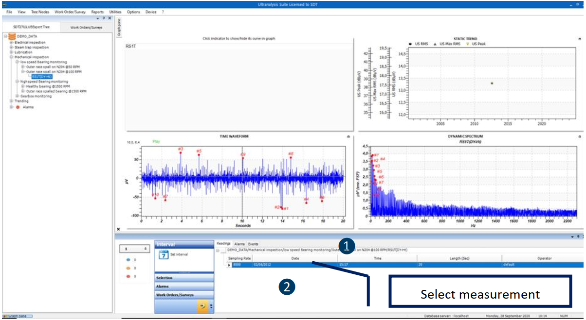
Graph Pane contains Matrix with recent measurements, Static Trend Graph, Time Domain and Frequency Domain, all of them essential tools for signal understanding and signal development monitoring. All available tools are powerful help in delivering actionable conclusions and still easy and practical in daily use. Here are the details about them.
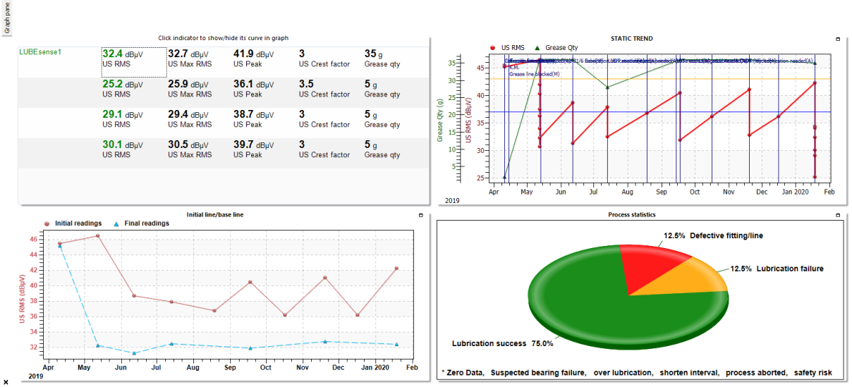
14.1. Matrix
Matrix shows four most recent readings, all four indicators (RMS, maxRMS, Peak and Crest Factor) for Ultrasound and Vibration and additionally, Added Grease quantity for LUBEsense1 sensor (LUBExpert and SDT 270 with LUBExpert features).
Reading data is sorted from most recent to oldest, top to bottom.
Each Ultrasound and Vibration indicator is being displayed in color corresponding with alarm status, as in picture below:
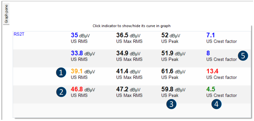
❶ Alarm assigned and in Warning status
❷ Alarm assigned and in Danger status
❸ Alarm NOT assigned
❹ Alarm assigned and NOT triggered
❺ Alarm assigned and in Alert status
By right clicking on indicator, you hide or show it in Static Trend Graph, focusing on indicator most important for the purpose of analysis.
14.2. Static Trend Graph
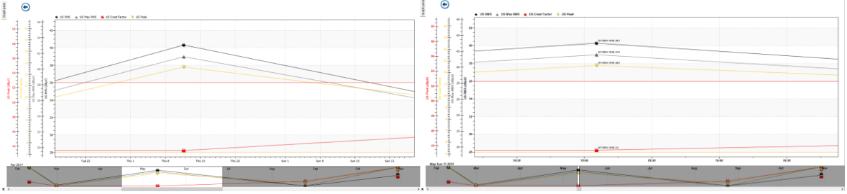
Static trend graph plots reading values in respect to time they were collected. It can be understood as a plot describing behavior in time. Values being table, trending down or trending up, are essential information for understanding asset health. Static Trend Graph contains lots of information and can be easily customized. Here is an example of static Trend Graph, so we can explain all details:

❶ Click to enlarge
❷ Events
❸ Events
❹ Y axis - amplitude for each displayed indicator, (auto scaled or Ymax defined)
❺ Trend line for each indicator
❻ Data points
❼ Alarm level
❽ X axis - time

❶ Font color of indicator on Y axis
❷ Corresponds with trend line of that indicator
You can customize your Graphs.
14.2.1. Define reading data to display
Left click on Options and then Graph & Static Trend settings in top toolbar, as shown in picture below:
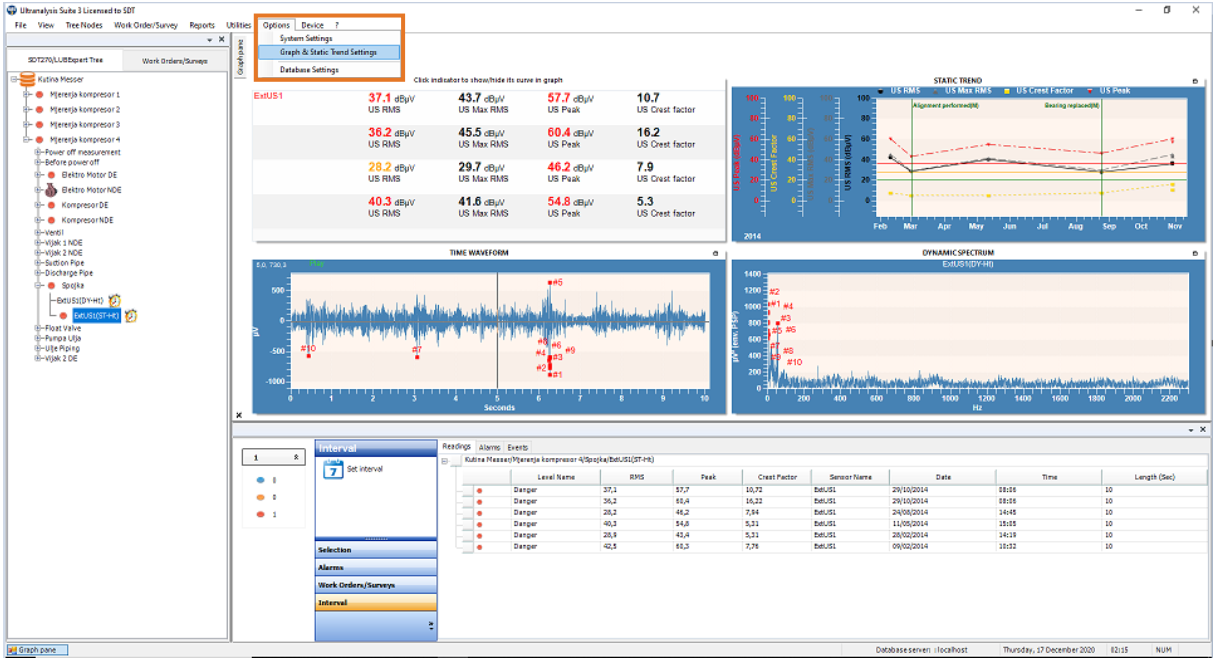
Graph & Static trend – Default Options window will pop up:
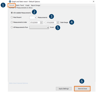
❶ Select tab General
❷ All available data will be displayed
❸ Most recent X readings will be displayed
❹ Only readings in defined date range will be displayed
❺ Only readings since selected interval will be displayed
❻ Confirm settings
14.2.2. Define Static Trend visual & Y scale settings
Left click on Options and then Graph & Static Trend settings in top toolbar and Graph & Static trend – Default Options window will pop up.
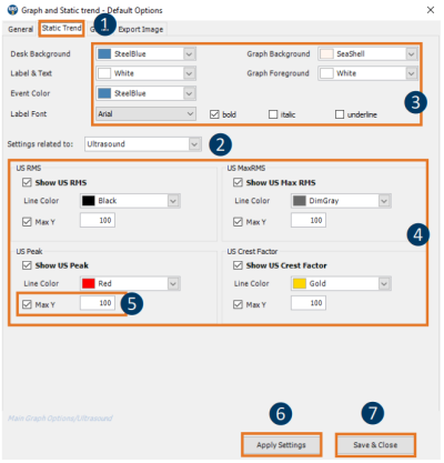
❶ Select Static Trend tab
❷ Select readings type (Ut, Vib, TEMp …)
❸ Select color scheme
❹ Select color for each indicator
❺ Define Y scale
- If left unchecked, Y axis will auto scale
- If checked, max Y value needs to be defined and scale will be displayed from -15 to “defined value” dBµV
❻ Apply selected settings
❼ Save settings and close the menu
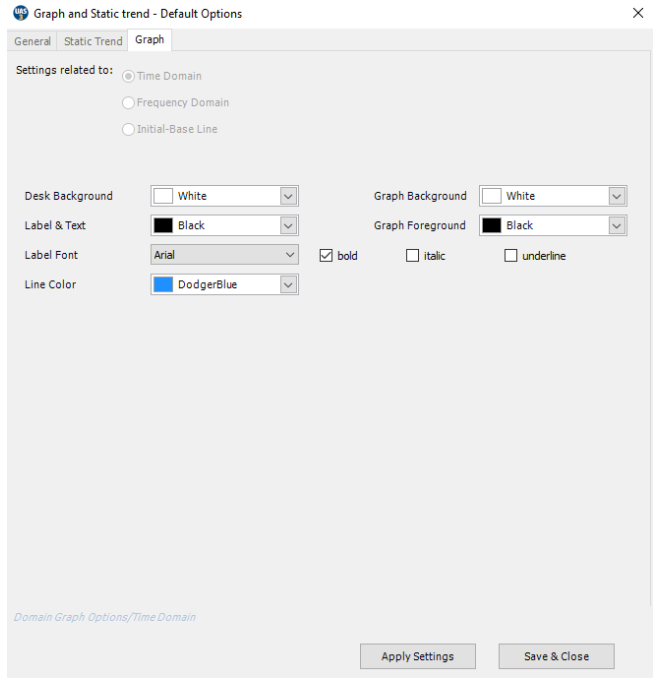
14.2.3. Define basic visuals of Time Domain, Frequency Domain and Initial-Base Line graph
This menu allows you to set up a visual for each of mentioned graphs:
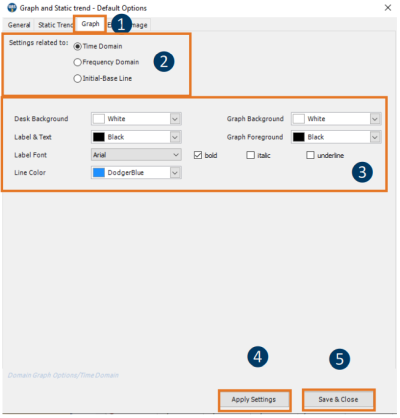
❶ Select Graph tab
❷ Select type of the graph you want to apply settings to
❸ Select color scheme
❹ Apply selected settings
❺ Save settings and close the menu
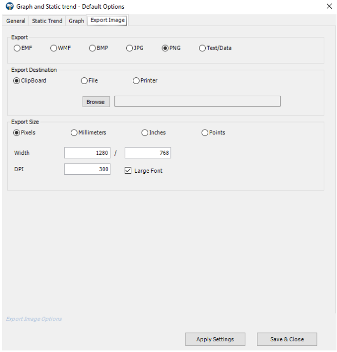
14.2.4. Define preferred settings for image export (Graph export)
This menu allows you to save your preferred setting for image export. Once you select exporting image, those settings will be offered as default, but you can still change them in export menu
14.2.5. Zoom
Place mouse pointer in graph and scroll mouse wheel to zoom in and zoom out. Zoom bar at the bottom of the graph shows you where the part of the graph you are looking at is positioned in entire graph. Hold non shaded part and move it left and right to dee other parts of the graph.
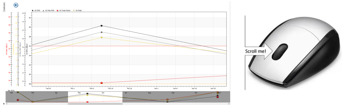
Another way to zoom in is to hold left click on your mouse and drag to form a rectangle. Selected area will be displayed. To zoom out, use mouse wheel.

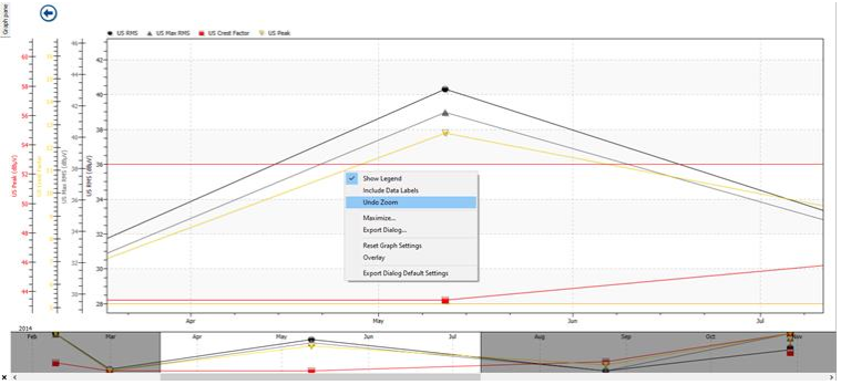
To undo zoom and go back to original full view, right click within the graph area, and choose Undo Zoom function, as below:
14.2.6. Show/Hide Labels
Labels, containing date, time, and value for each datapoint can be shown or hidden. Right click anywhere within graph area and select Include Data Labels.
14.2.7. Maximize
Right click anywhere in the graph area and select Maximize; graph will be displayed full screen. To exit full screen, press esc or click in top left corner of the graph.
14.2.8. Export graph
Right click anywhere in the graph area and select Export Dialog; Export Control window will pop up.
Choose your settings and export graph.

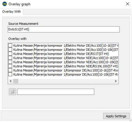
14.2.9. Overlay Graph
Right click anywhere in the graph area and select Overlay; Overlay Graph window will pop up.
Choose the measurement point you want to overlay with current graph, choose indicators to show and confirm settings. To cancel overlay, follow the same path and uncheck selected overlay measurement points.
14.2.10. Accessing settings menu directly from graph
Left double click within the graph, and you will access settings menu directly. When settings assessed directly from the graph, it is locked to that graph type. That means that change is possible for that type only. Same shortcut is available for following graph types: Time Domain, Frequency Domain, Static Trend and Initial-Base line in case of Lubrication.
14.3. Time Domain Graph
Time Wave Form is fundamental way of representing an event collected through Dynamic measurement. It plots amplitude in time, thus giving us a clear view on what happened and when.
Select the measurement you want to see and click on enlarge.

❶ Click to enlarge
❷ Select measurement
Time Domain window will be enlarged, and all Time Domain tools will be displayed and active:

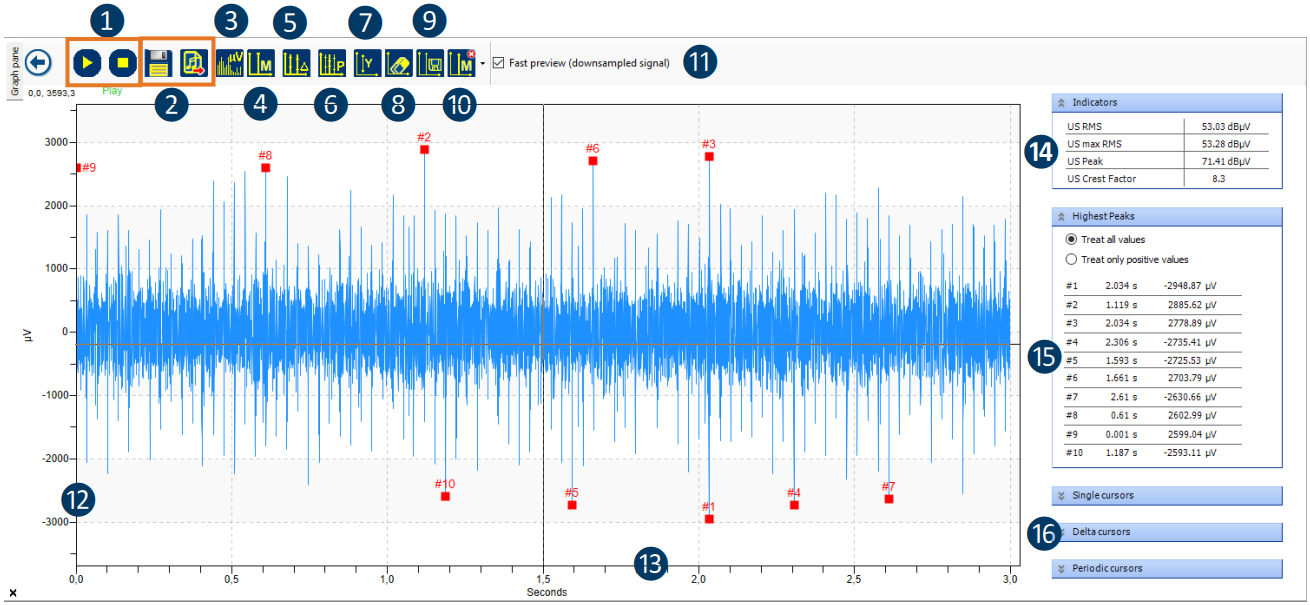
❶ Play and stop audio
❷ Export signal/export audio
❸ Frequency domain
❹ Add single cursor, comment
❺ Delta cursor
❻ Periodic cursor
❼ Set Y scale
❽ Delete portion of the signal
❾ Save cursors
❿ Remove cursors
⓫ Graph sampling
⓬ Y axis, amplitude in µV
⓭ X axis, time
⓮ Indicators for selected signal
⓯ List of highest peaks in signal
⓰ Cursors details
14.3.1. Play Audio
Left click on Play to listen to audio and Stop to stop it. Green line will visually indicate progress, so you can connect what you hear and what you see in the signal.
14.3.2. Export Wav File
Left click on Save icon and export wav file/audio of selected reading.
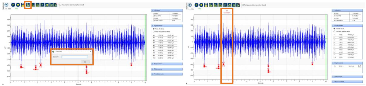
14.3.3. Add Single Cursor/Comment
Left click on indicated tool, and Comment window will pop up, add comment, and left click in signal area to add comment. Move comment to other position if necessary, by holding left click, moving it to new position and release.
14.3.4. Add Delta Cursor
Left click on indicated tool, then left click in signal area to place the cursor. Move D1 (lead cursor) to needed position and move D2 to define ∆. In a signal descriptor on the right side, cursor details will be displayed; position in time, amplitude, ∆t (time) and corresponding ∆f (frequency)

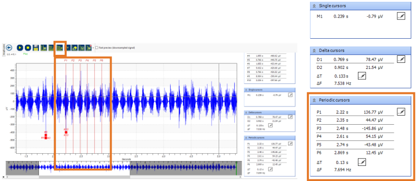
14.3.5. Add Periodic Cursor
Left click on indicated tool, then left click in signal area to place the cursor. Left click and hold on P1 to move it to needed position, then left click and hold any of other cursors (P2-P6) to adjust the ∆t.
Alternatively, set both P1 position and ∆t in cursor details on the right side. Cursor details display; position in time, amplitude, ∆t (time) and corresponding ∆f (frequency).
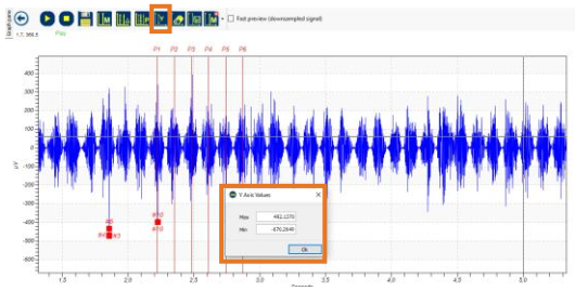
14.3.6. Set Y Scale
This tool allows you to set Y scale, for purpose of comparison or overlaying graphs. Left click on indicated tool, and Y Axis Values window will pop up. Set Y scale and confirm by pressing Ok.
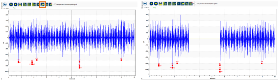
14.3.7. Delete Portion of the Signal
This function enables you to temporarily delete potion of the signal (by delete, meaning is that selected portion is set to amplitude zero), for the purpose of analysis. Indicators will automatically be recalculated based on new TWF values. Zoom on portion of the signal you want to delete and press on indicated tool. Note, deleted portion of the signal will be exactly that on the screen. By selecting any other measurement and coming back to the processed signal, delete action will be reverted.
14.3.8. Save Cursors
This function allows you to save cursors you have set in TWF.
14.3.9. Remove Cursors
This function allows you to remove individual cursor (click on small arrow on right side of the tool), or all cursors.
14.3.10. Indicators for Selected Signal (TWF)
This window display indicators (RMS, maxRMS, Peak and Crest Factor) for selected TWF.
14.3.11. List of highest Peaks in Signal
This window displays 10 highest Peaks in selected TWF, in descending order. You can choose to display all values or only positive values.
14.4. Frequency Domain Graph
The Frequency Domain Graph of Dynamic Measurement displays how much of the Dynamic Measurement lies within each given frequency band over a range of frequencies. Select the measurement you want to see and click on enlarge.
❶ Click to enlarge
❷ Select measurement
Frequency domain window will be enlarged, and all tools will be displayed and active:

❶ Export wav file
❷ Switch to TWF
❸ Single cursor
❹ Delta cursor
❺ Periodic cursor
❻ Comment
❼ Set Y scale
❽ Save cursors
❾ Remove cursors
❿ Y axis,
⓫ X axis, frequency
⓬ Indicators for selected signal
⓭ List of highest peaks in signal
⓮ Cursors details
All tools operate the same way as they do in Time Domain.
14.5. Specific LUBExpert Graphs
For detailed manual about specific functions of LUBExpert feature in UAS3, please refer to LUBExpert Manual.